Introduction

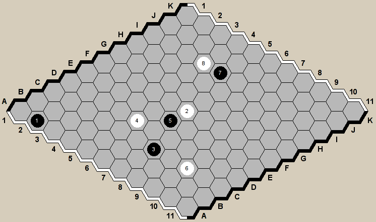
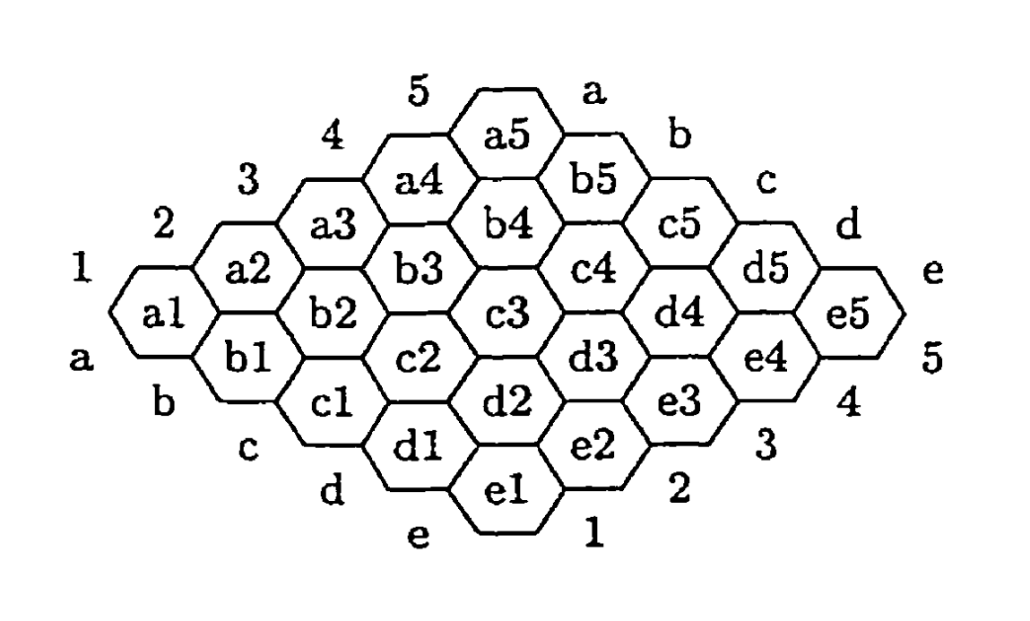
Hex is a classic strategy board game, first invented by Danish mathematician Piet Hein in 1942 and independently rediscovered by John Nash at Princeton University in 1948. The game is played on a diamond-shaped hexagonal grid, typically 11x11 or larger. Hex’s rules are simple and straightforward, yet its strategy is profoundly complex, making it an ideal platform for research in artificial intelligence and game theory.In this paper, for ease of discussion and demonstration, we utilize a 5x5 board and employ the board coordinates as shown in Figure 2.

The game involves two players, each using black and white pieces. Players take turns placing their pieces on empty cells, aiming to connect their respective colored edges with an unbroken chain of pieces. A notable feature of Hex is that the game cannot end in a draw, ensuring that one player will inevitably win each match.

The complexity of Hex lies not only in its deep strategy under simple rules but also in its close ties to graph theory. In fact, Hex is a special case of the Shannon switching game, which has been proven to be PSPACE-complete. This indicates that decision-making in Hex is computationally challenging, especially as the board size increases.

In this paper, we propose a novel algorithm designed to enhance decision-making capabilities in Hex for computer players. By integrating advanced search techniques and evaluation strategies, our algorithm demonstrates exceptional performance across various board sizes, showcasing its potential application in Hex gameplay.

Queenbee’s Evaluation Function

A game program requires a good evaluation function to guide its search. However, for the game of Hex, constructing a meaningful evaluation function is not immediately obvious. For example, unlike many other board games, the concepts of material balance and mobility are completely useless in Hex. This chapter contains some new ideas about the evaluation function for Hex, which have been implemented in the Hex program Queenbee. The function calculates the distance from all unoccupied cells on the board to each edge based on an unconventional distance metric called “two-distance.” The resulting distances are referred to as “potential.”

Two-Distance

Given a graph $ \Gamma $ with an adjacency function $ n(p) $ that maps a vertex $ p $ to the set of vertices adjacent to it, there is a distance metric $ d_z $ to generalize the traditional distance metric:

$$d_z(p, q) = \begin{cases} 0 & \text{if } q = p, \\ 1 & \text{if } q \in n(p), \\ \min_k c_k(p) \geq z & \text{otherwise}, \end{cases}$$

where

$$c_k(p) = \{ r \in n(p) | d_z(r, q) < k \}.$$

The traditional distance metric corresponds to $ z = 1 $, in which case the distance from a cell to an edge represents the number of “free moves” a player needs to connect the cell to a given edge. Unfortunately, this distance function is not very useful for constructing an evaluation function for Hex. Instead, the concept of two-distance is used.

The image below shows the distance from each cell on a 5x5 board to the lower black edge, according to these two metrics. The intuition behind two-distance is that in the game, one can always choose to force the opponent to choose a suboptimal option by blocking the best choice. Consider e4, the cell with boxed numbers in the image. The traditional distance indicates that it takes only four steps directly to the lower black edge. However, only one path from e4 achieves this distance. In contrast, the two-distance equals because the best two adjacent connections have distances of 5 and 6. Two-distance thus captures the essence of “suboptimal choices.”

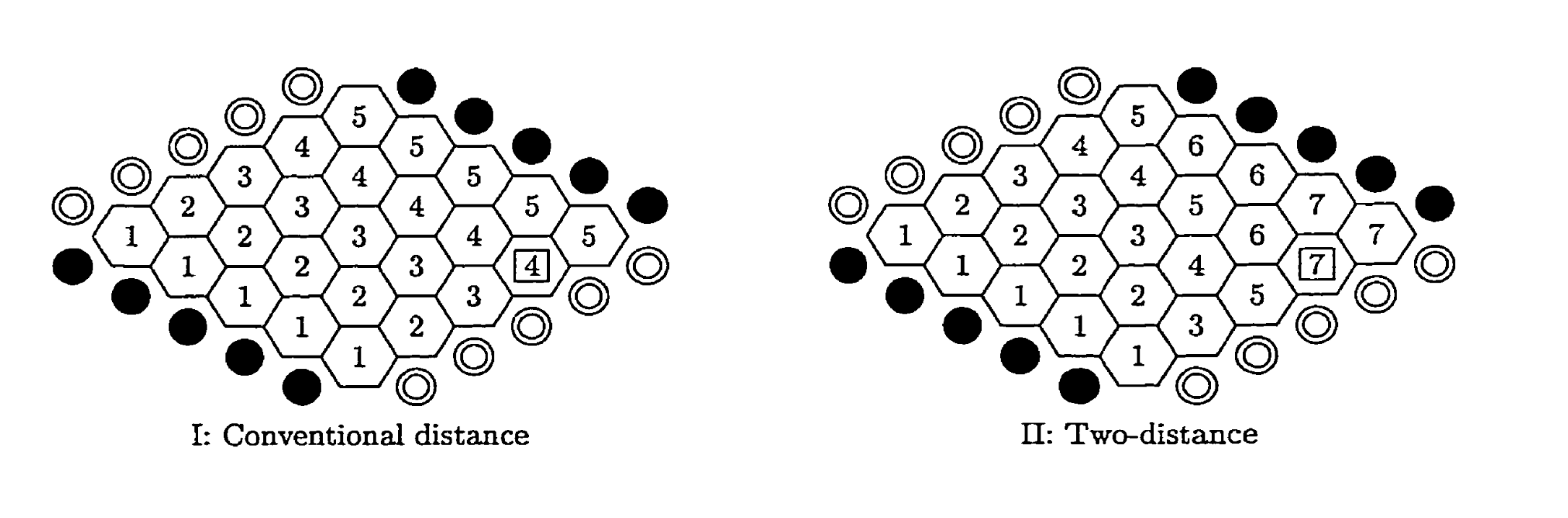
Note that the two-distance for the rightmost cell e5 on the board is 7, even though its directly adjacent neighbor also has a two-distance of 7. This number is still correct because calculating two-distance requires considering the entire neighborhood. Adjacency implies neighborhood, but not vice versa. Two cells are adjacent if they share a common edge. The concept of neighborhood considers the black and white stones already present on the board. Two unoccupied cells are neighbors from the perspective of white stones if they are adjacent or connected by a string of white stones.

Note that a cell’s neighborhood can differ from the perspective of white stones. These two neighborhoods will be referred to as W-neighborhood and B-neighborhood, respectively. Accordingly, W-distance and B-distance will be distinguished. This explains why the two-distance from cell e5 to the lower black edge is 7; due to edge stones, its B-neighborhood includes cells a5 and b5, with distances of 5 and 6, respectively.

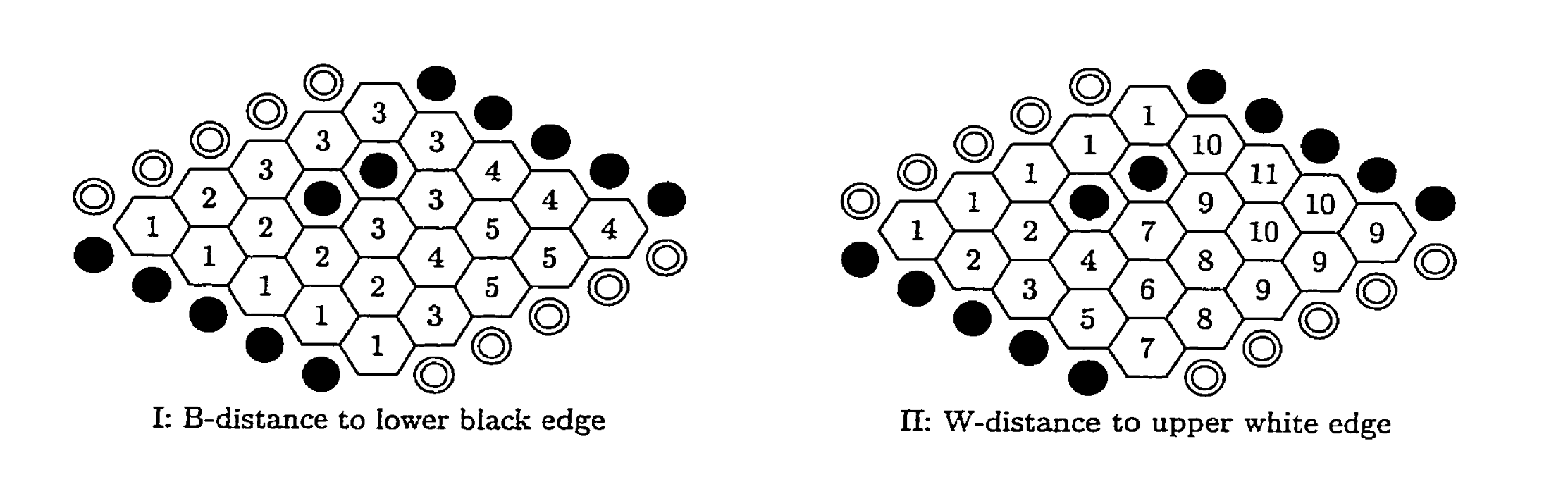
In Figure 5.2, two black stones have been added. Figure 5.2-I shows the B-distance from unoccupied cells to the lower black edge, and Figure 5.2-II shows the W-distance to the upper white edge. Adding these two black stones causes, for example, cells c2 and b5 to become B-neighbors but not W-neighbors.

Potentials

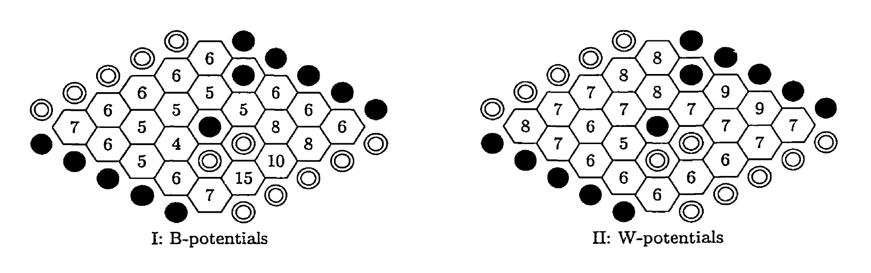
The goal in Hex is to connect two sides of the board. To help achieve this, one might look for an unoccupied cell that is as close as possible to being connected to both sides, as this would be a promising candidate for being part of a winning chain. The evaluation function calculates potentials that capture this concept. Each unoccupied cell is assigned two potentials, based on the two-distance metric. A cell’s W-potential is defined as the sum of its W-distance to both white edges; its B-potential is the sum of its B-distance to both black edges. Figure 5 shows the potentials for a position with two white and two black stones on the board.

Cells with low W-potentials are the ones that are closest to being connected to both white borders by White. If White can connect a cell to both white borders, this would establish a winning chain. White will therefore focus on those cells that have the lowest W-potentials. The white board potential is defined as the lowest W-potential that occurs on the board. In the example of Figure 5, the white board potential is 5, and the black board potential is 4. As lower potentials are better, it appears that Black is ahead.

In the same figure, it can be seen that both Black and White have only one cell that actually realizes their board potential. For both players, it is the cell c2. It would be better to have more than one cell that realizes the board potential, so as to have more attack options and be less easy to block. The attack mobility is defined for each player as the number of cells that realize that player’s board potential.

Queenbee’s evaluation function uses only the two concepts of board potential and attack mobility. The evaluation function returns the following number:

$$e = M(p_B - p_W) - (a_B - a_W)$$

where:

• $ p_W $ = white board potential;
• $ p_B $ = black board potential;
• $ a_W $ = white attack mobility;
• $ a_B $ = black attack mobility;
• $ M $ = a large number.

If $ M $ is set to be sufficiently large, the evaluation function will prefer one position over another if its board potential difference is better, and only use the attack mobility difference as a tie-breaker for positions with equal board potential difference. The potential of a cell, if it is finite, cannot be larger than $ 2n^2 $ on an $ n \times n $ board. Therefore, using a value for $ M $ of the order of magnitude of $ n^2 $ will achieve this. In our work, we use $ M = 100 $.

Game Tree

In the game of Hex, while Queenbee’s evaluation functions provide immediate value judgments for specific situations, they are limited to static analysis of the current state. To make more comprehensive and strategic decisions, the use of game trees is essential. Game trees allow us to simulate sequences of possible future moves, thereby predicting the opponent’s responses and potential game progress. By combining game trees with evaluation functions, players can identify the best moves by exploring the tree, comparing the outcomes of different strategies, and choosing those that maximize their chances of winning.

A game tree is a structure used to simulate possible future sequences of moves in a game. By constructing a game tree, players can anticipate the opponent’s responses and the potential progression of the game. Each node represents a game state, while the edges represent possible moves from one state to another.

Minimax Algorithm

The Minimax algorithm is a classic decision-making algorithm, particularly suited for zero-sum games. Its basic idea is to maximize the player’s minimum gain, assuming the opponent will make the most detrimental choices for the player. The pseudocode is as follows:

function minimax(node, depth, maximizingPlayer):
    if depth = 0 or node is a terminal node:
        return the heuristic value of the node
    if maximizingPlayer:
        bestValue = -infinity
        for each child node of node:
            v = minimax(child, depth - 1, FALSE)
            bestValue = max(bestValue, v)
        return bestValue
    else:
        bestValue = +infinity
        for each child node of node:
            v = minimax(child, depth - 1, TRUE)
            bestValue = min(bestValue, v)
        return bestValue

Alpha-Beta Pruning

Alpha-Beta pruning is an optimization technique for the Minimax algorithm, aimed at reducing the number of nodes that need to be evaluated, thereby improving efficiency. The basic principle is to prune unnecessary branches, avoiding the evaluation of moves that are clearly disadvantageous. The specific steps are as follows:

• Alpha value: Represents the minimum score that the current player is assured of.
• Beta value: Represents the minimum score that the opponent is assured of.
• Pruning condition: If at any node, the Beta value is less than or equal to the Alpha value, further evaluation of that node can be stopped, as the opponent will not choose that path.

Through Alpha-Beta pruning, the algorithm can skip a large number of unnecessary calculations without affecting the final decision, significantly improving efficiency. This is particularly important for complex games like Hex, where the number of possible states grows exponentially with the board size. The pseudocode is as follows:

function alphabeta(node, depth, α, β, Player)         
    if depth = 0 or node is a terminal node  
        return the heuristic value of node  
    if Player = MaxPlayer  
        for each child of node  
            α := max(α, alphabeta(child, depth-1, α, β, not(Player)))  
            if β ≤ α  
                break  
        return α  
    else  
        for each child of node  
            β := min(β, alphabeta(child, depth-1, α, β, not(Player)))  
            if β ≤ α  
                break  
        return β

Experiment

To evaluate the performance of our algorithm, we conducted experiments on the Botzone platform. Due to time constraints, we did not perform an exhaustive search for optimal hyperparameters. Instead, we used heuristic methods to select parameters suitable for an 11x11 board. Following the initial setup, we uploaded our Bot to the competition platform under the ID 6266ba6e351b6f7f90682672, where users can search for this ID to engage in matches.

Discussion

After achieving promising initial results, we plan to further optimize the algorithm to enhance its performance on larger board sizes. Our future work includes:

• Hyperparameter Optimization: A more systematic approach to adjusting hyperparameters, aiming to discover potentially superior configurations.

• Incorporating Machine Learning: Exploring the integration of machine learning techniques to allow the algorithm to autonomously learn optimal strategies and improve decision-making.